CS280A Project 4

Image Warping and Mosaicing

Name: Cyrus Vachha (cvachha@berkeley.edu)

Introduction: Project 4A

In this project we create panoramas by applying perspective projection transformations on multiple images (taken at a similar center of projection) and overlay them to fit them to a single projection plane to create wide angle panoramic images.

Part 1: Shoot the Pictures

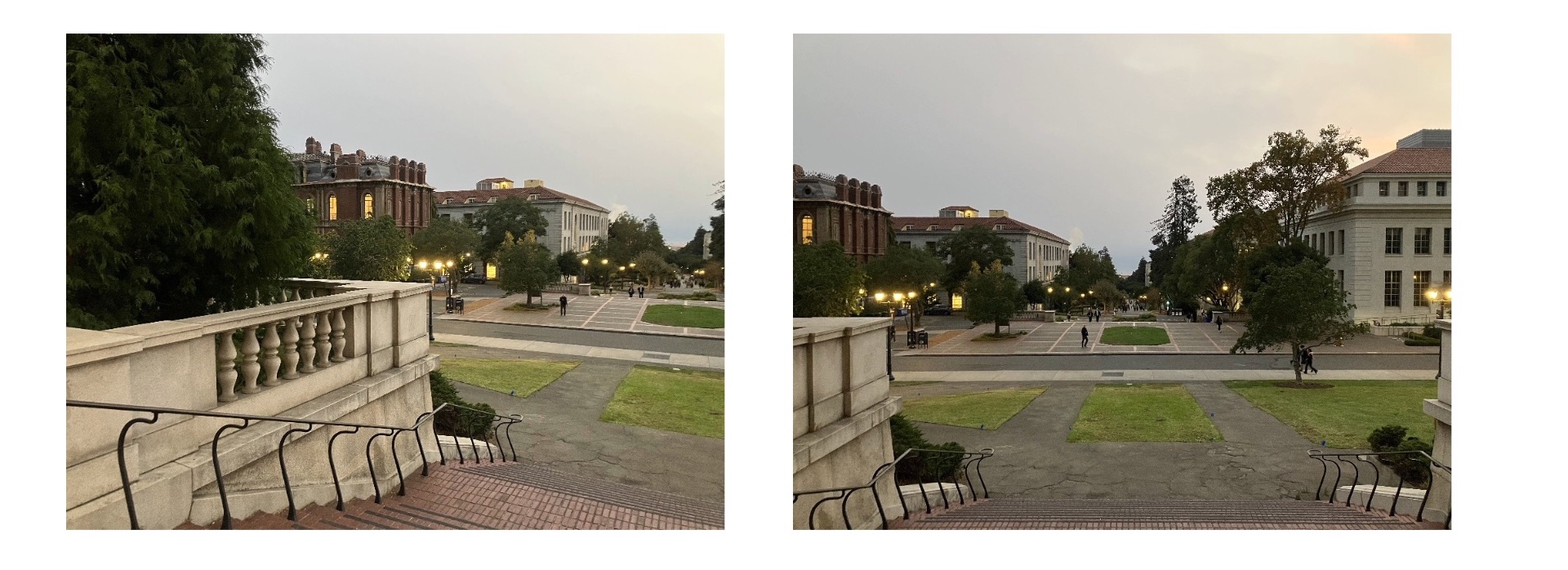
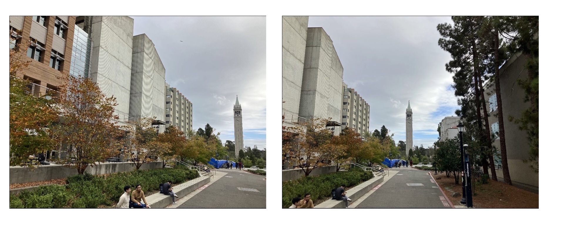
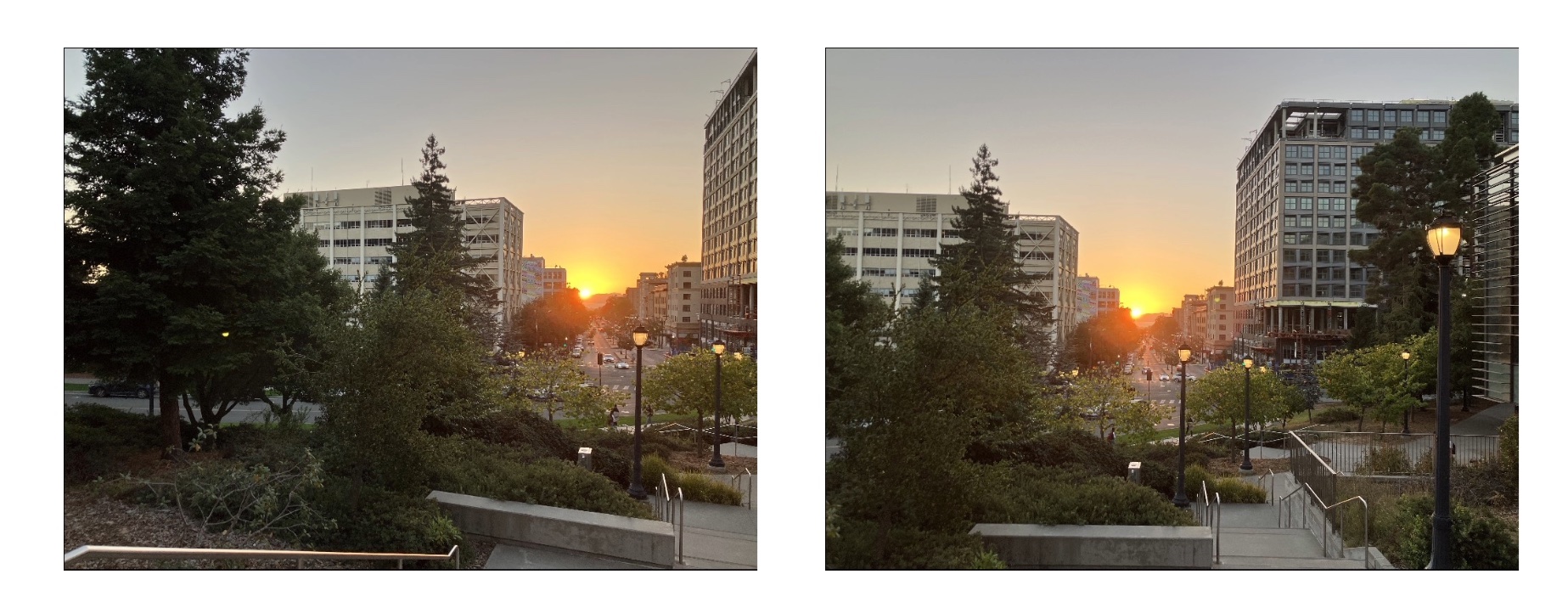
I took a few sets of images for the panorama stitching where I rotated the camera in place.

Campanile base

Walkway

Sunset

Part 2: Recover Homographies

To recover the homographies, I first found the corresponding points across the images hand-selected using the correspondence tool from Project 3 and used multiple points for each set of images to ensure that I get a reasonable warp. The homography matrix would be needed to transform the points from the first image to the second image to have both images projected on the same image plane to appear as a large photo mosaic panorama.

To calculate the homography matrix with points p and p’, I compute the H matrix in the equation: p’ = Hp which is a 3x3 matrix. I then used matrix operations and system of equations to assemble a least squares equation of Ah = b where A is the matrix of the points in expressions, h is the homography matrix, and b is the transformed points. I used the np.linalg.lstsq function to solve for h and verified the accuracy by transforming and reverse transforming the points.

Part 3: Warp the Images

Then I created a warp image function similar to the warp triangle function in Project 3. I first found the corners of the input image, warped those with the homography matrix, and then used the poly function to find the points in that area. I then performed inverse warping and was able to reconstruct the warped image with pixel color samples from the original image. I tried pixel sampling with interpolation but it took significantly longer so I disabled it when testing. I noticed that manually selecting the correct points accurately was essential to have a resonable warp. I also had to account for pixel offsets when performing the transformations, so I used cv2.boundingRect.

Part 4: Image Rectification

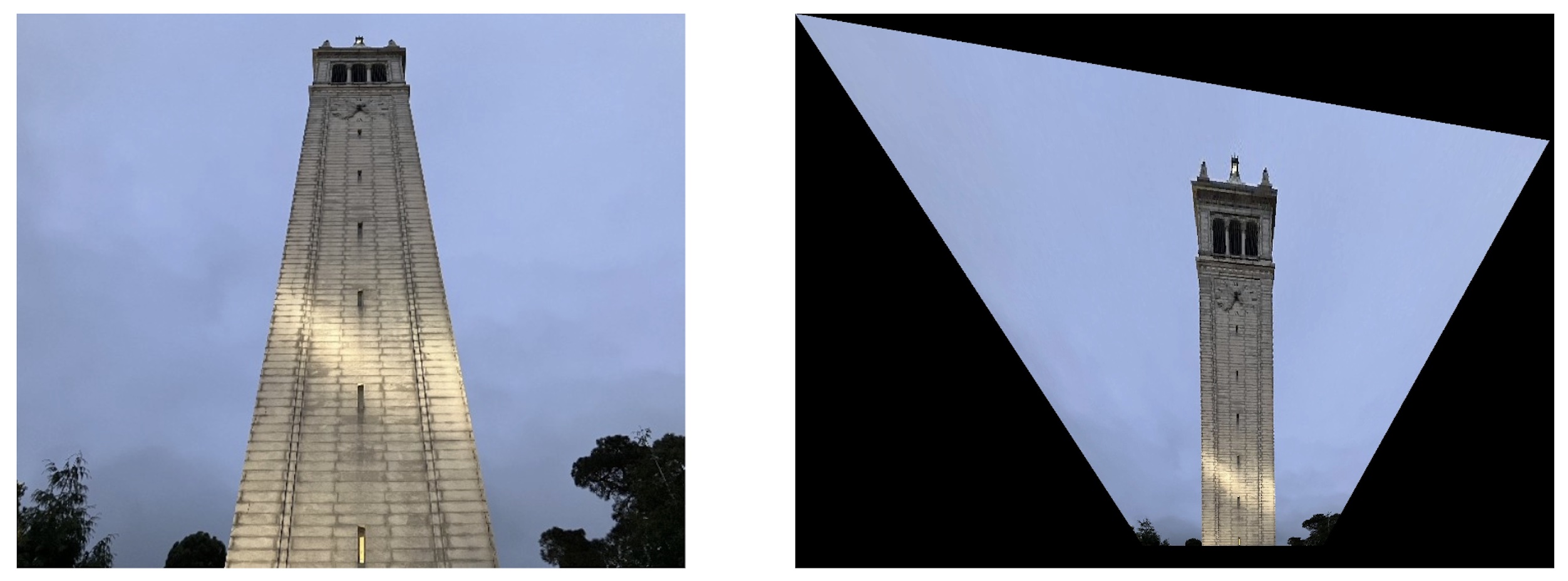
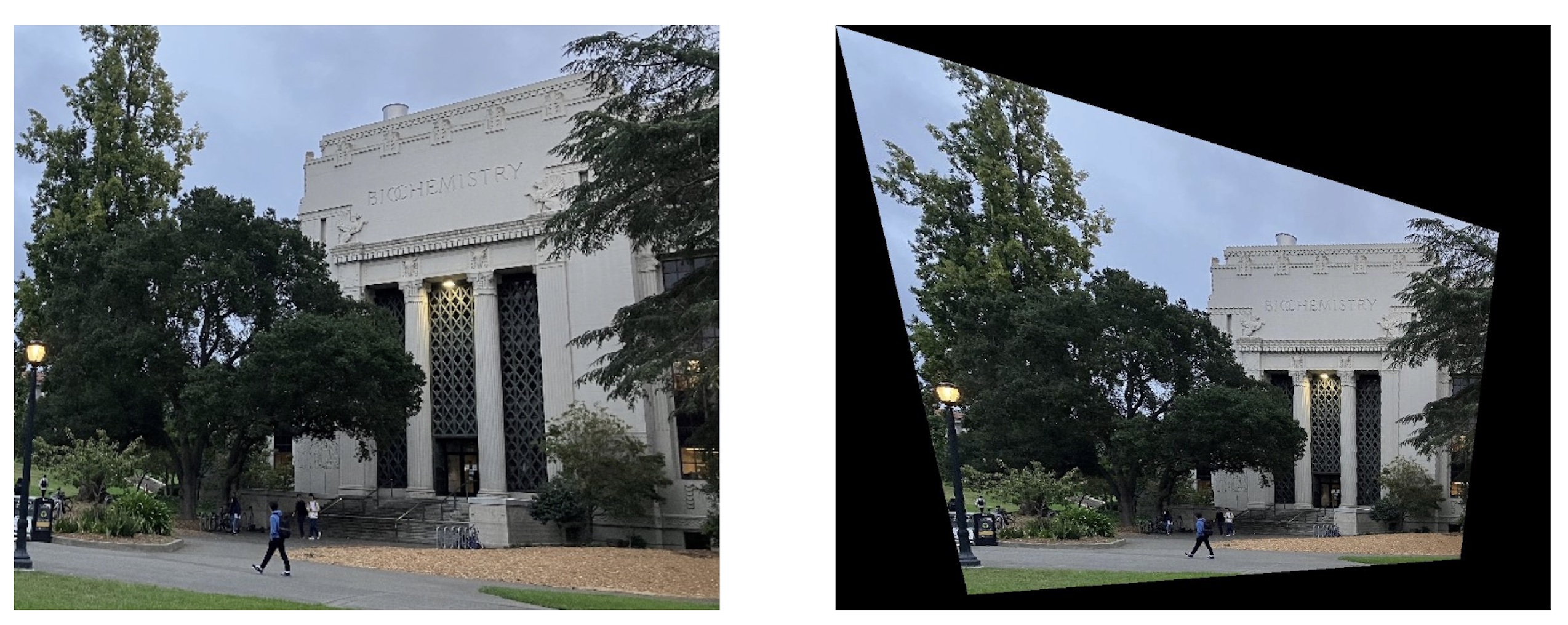
After creating the warp image function, I tested this with other images to “flatten” parts of the image (planar surfaces) taken at different perspectives. I manually selected corresponding points and also selected points that would make a square/rectangular region plane. I computed the homography between the points and warped to rectify the images.

Campanile rectification

VLSB rectification

Part 5: Blend the images into a mosaic (manual correspondences)

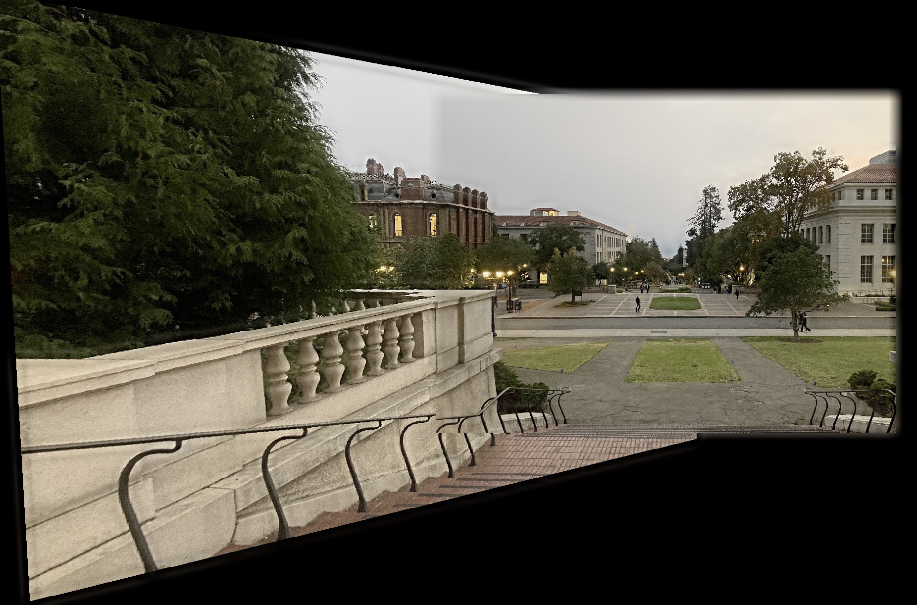
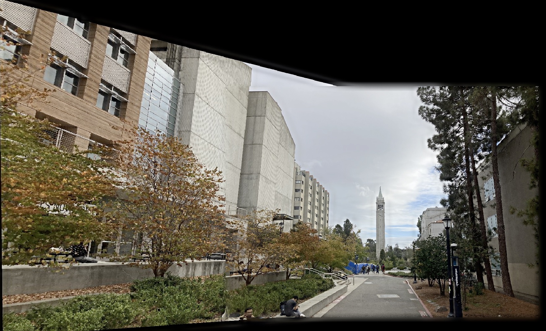
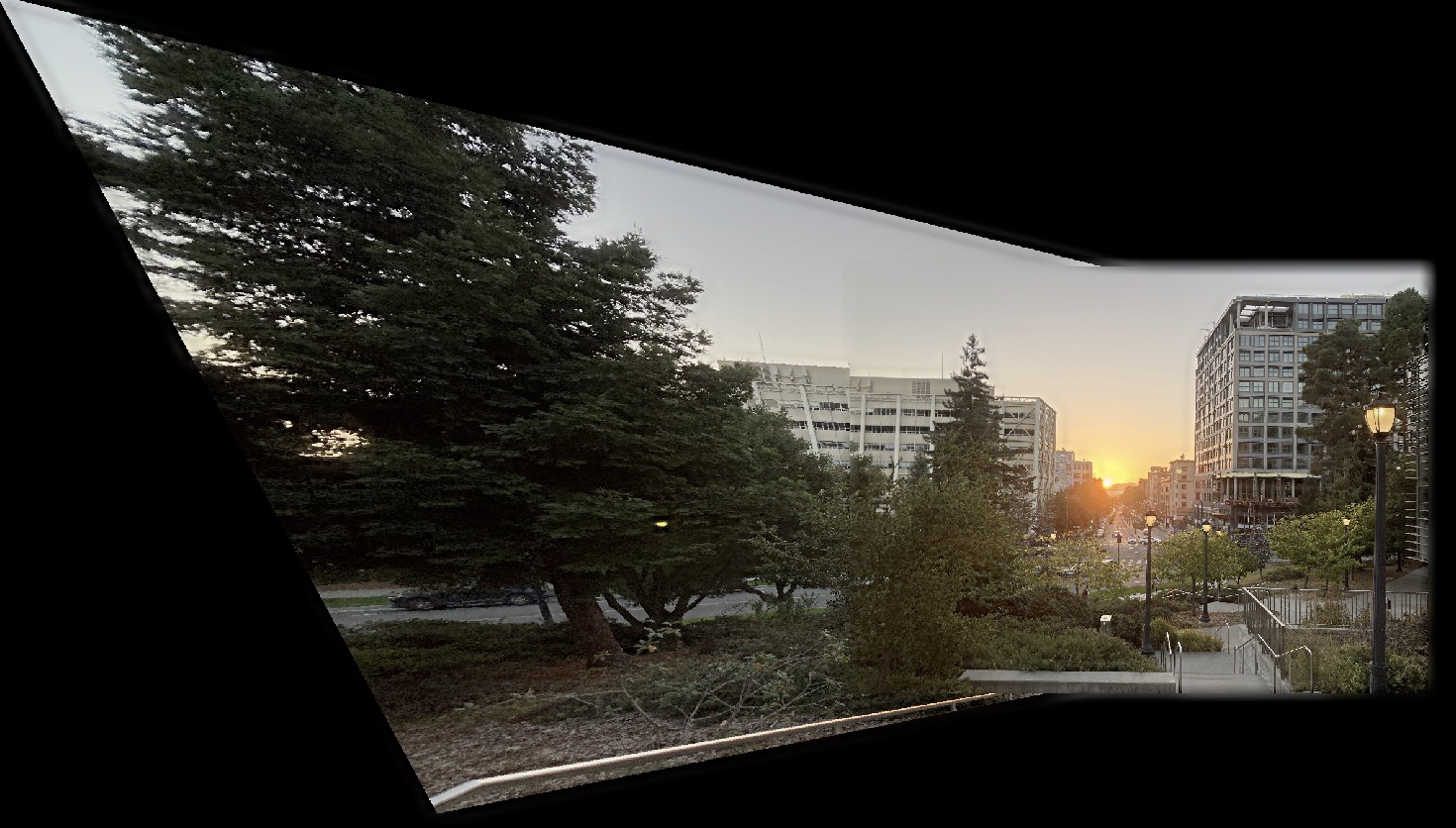
Once I created the warped images for each panorama sub image based on the homographies, I then had to blend their edges so the panorama appears seamless. I did this by first getting each image individually, generating a mask, and blending two images at a time. The mask I used was based on the second image mask. I also experimented with applying dilation to the mask to improve smoothening.

Panorama Campanile Base

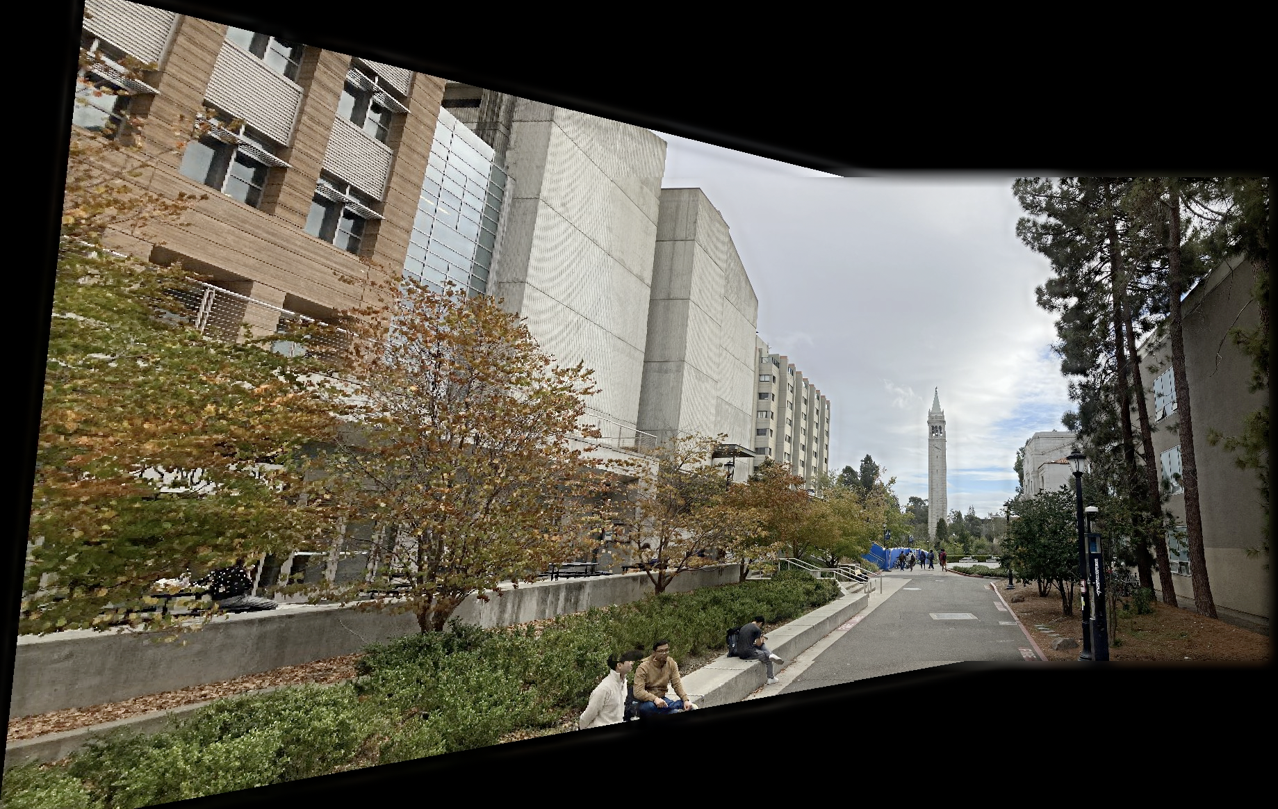
Panorama Walkway

Panorama Sunset

Reflection: Part A

I found this project interesting since I used to capture many spherical panoramas on my smartphone and was interested in knowing how they are implemented, so it is good to learn this. I also found it interesting that the panorama doesn’t look perfectly accurate since the objects in the scene are 3D and some parts occlude other parts, which is evident in the rectification of the campanile image.

Project 4B: Feature Matching for Autostitching

Introduction: Project 4B

In this part of the project, I automated the selection of corresponding feature points by implementing feature detection, matching, and use RANSAC to find the optimal feature points to create a homography matrix to automatically stitch the panoramic image. This project implements the 2005 paper Multi-Image Matching using Multi-Scale Oriented Patches by Brown, Szeliski, and Winder.

Detecting corner features in an image

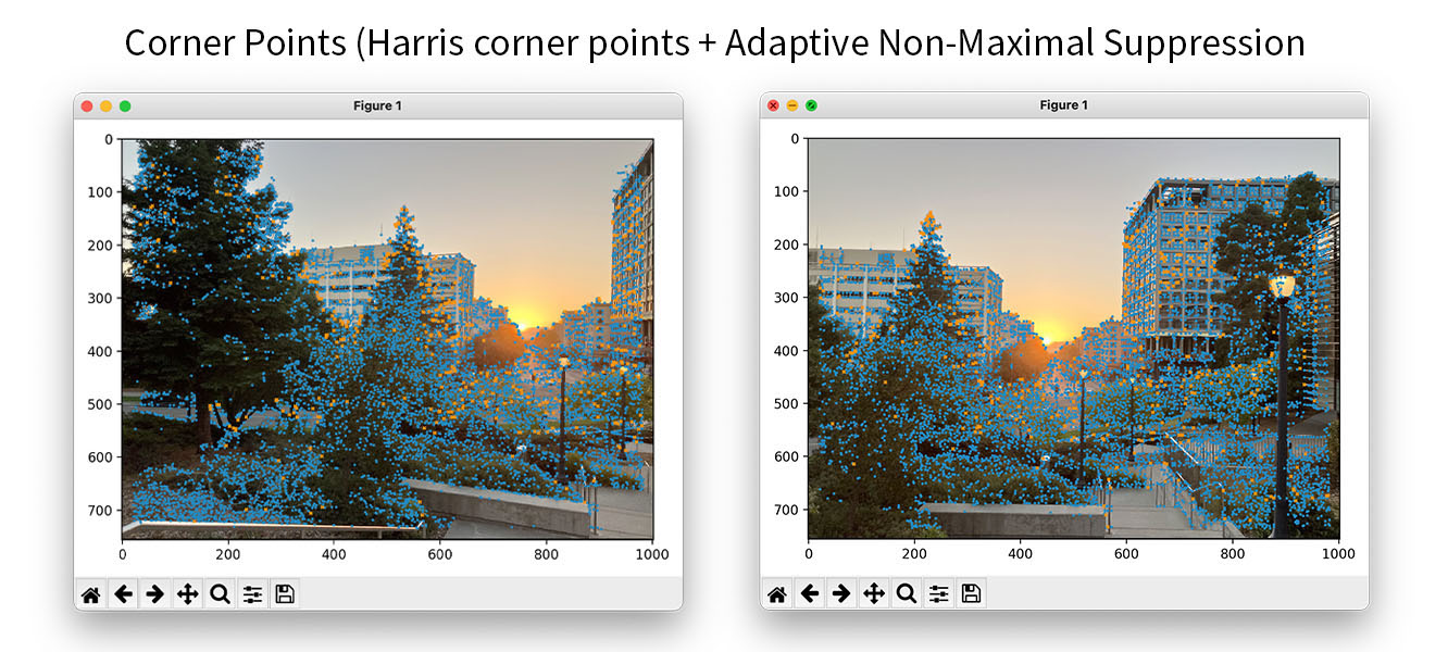
To start finding the feature points, I used the harris.py code to find the corners with the harris corners algorithm. I also adjusted the threshold_rel value to 0.01 which helped get slightly better corners than just everything. Since there are thousands of harris corner points are found per image, I implemented Adaptive Non-Maximal Suppression to choose the “best” 500 points. I needed to select the top 2500 points with the highest h-value since running Adaptive Non-Maximal Suppression on 10,000+ points would take hours to run. I chose these 500 points by comparing each feature point with every other feature point and found the minimum radius boundary where all points within that range satisfy the condition that h_starting_point > (0.9*p_other_point). From the list of chosen points, I chose the top 500 points with the greatest radius and made these the feature points.

This example shows the feature points from each input image. Blue points as the feature points found with harris corners and the orange points are chosen as the best 500 points from Adaptive Non-Maximal Suppression.

Extracting a Feature Descriptor for each feature point

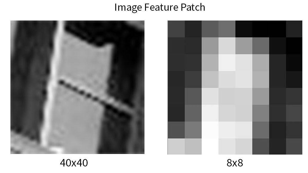
Now that we have got a selection of possible feature points in each image, I need to match each feature region in both images to find the correlations. To do this, I take a 40x40 pixel patch, downsample it to 8x8 and then bias/normalize it to prepare it to compare with the other image.

Here is an example of a feature patch.

Matching these feature descriptors between two images

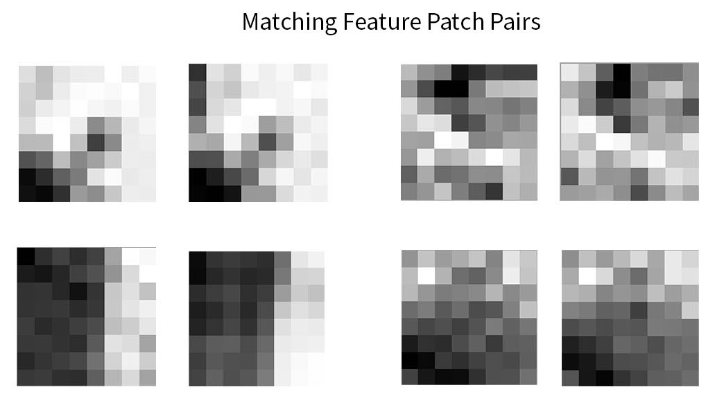
Once we have a set of feature patches for each image, I then matched the patches and find the best fit. To perform the matching, I find the two most closest matches to an image patch in the first image with a path in the second image with L2 loss. I then evaluate its effectiveness by thresholding the ratio of the 2 nearest patches as NN1/NN2 and if the ratio is small enough (since the closer the image is, the smaller the L2 loss is) this means that the nearest image patch is significantly enough different from the second image patch so it is more likely a true match. I accept these matches and construct the list of likely correspondences.

This figure shows pairs of matching image patches from image 1 and image 2. We can see that they appear very similar.

Using RANSAC to compute a homography

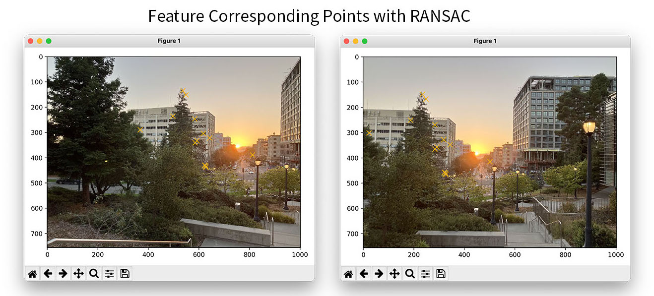
Once we have multiple feature points, I use RANSAC to find the best homography matrix and set of points that capture the best homography matrix. In this process, I randomly chose four sets of corresponding feature points and computed the homography matrix. I then applied this homography matrix to all the feature points in image 1 and counted the number of “inliers” where the points from image 1 correctly correlate to the found image 2 correspondences. I repeated this procedure 500 times to come up with a list of potential homography matricies and chose the best set of four corresponding points where there was the maximum number of inliers.

Here are the feature correspondences found by RANSAC.

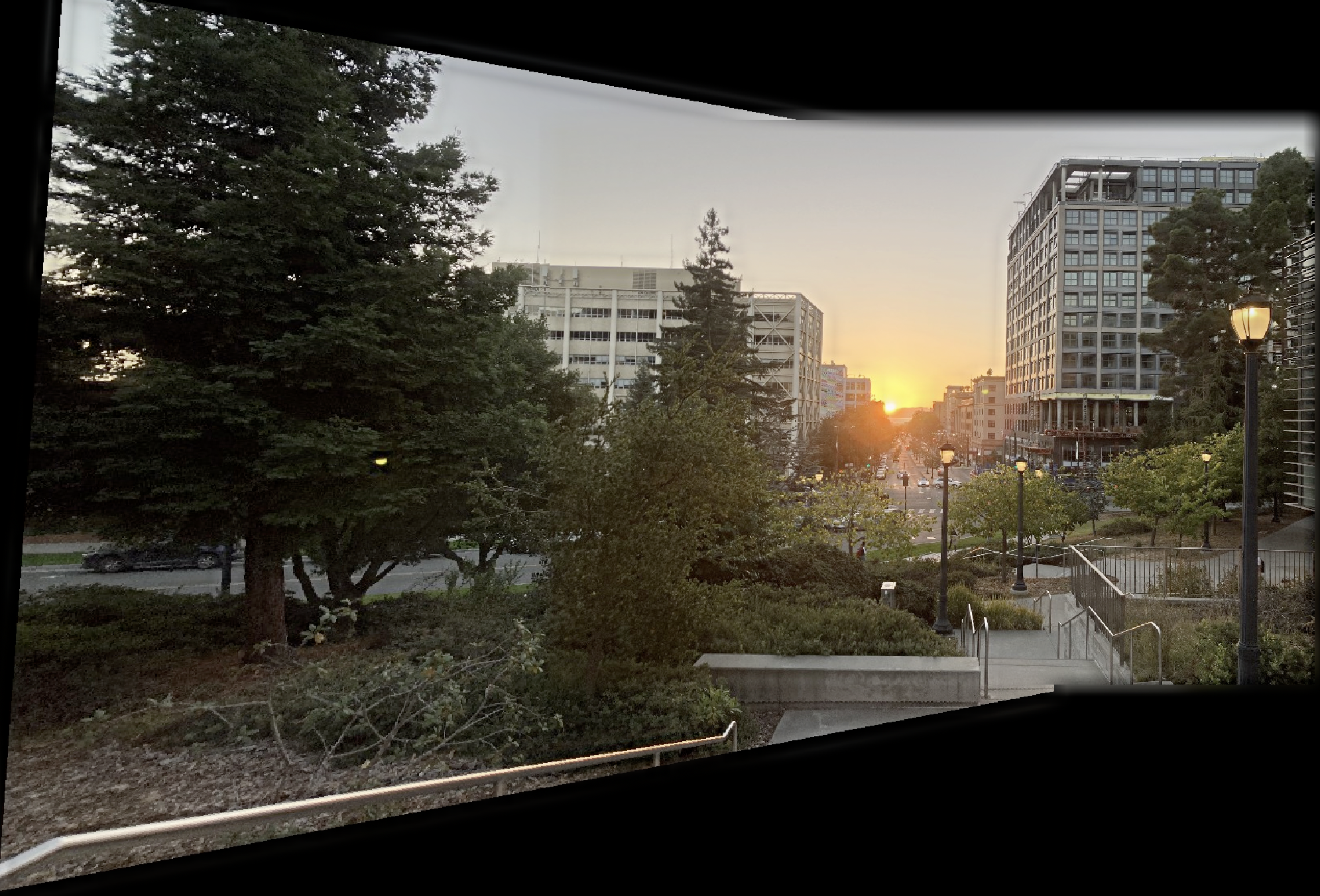
Finally, I apply these corresponding points and proceed with the original panorama image blending system and create the final blend images.

Sunset

Campanile Base

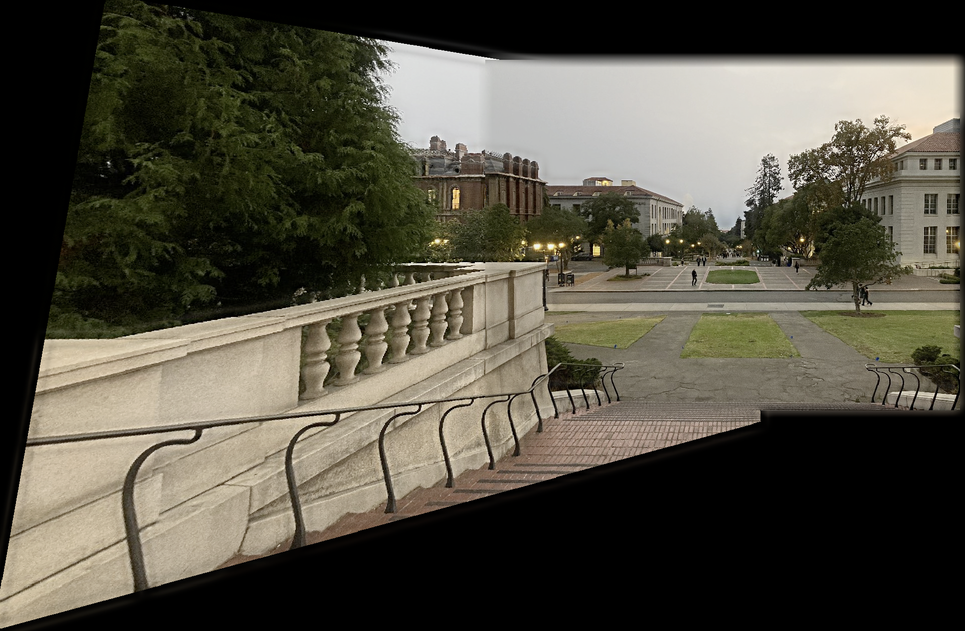
Walkway

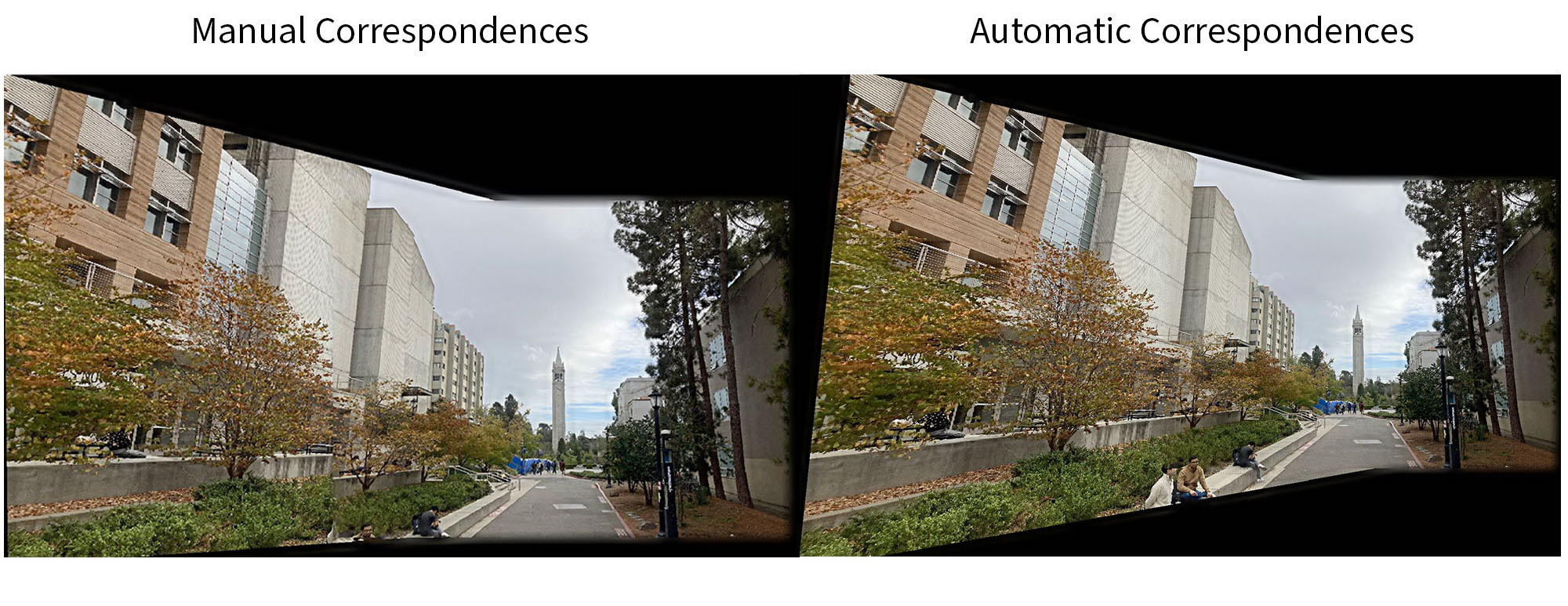
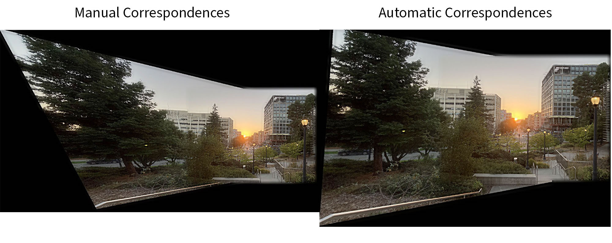
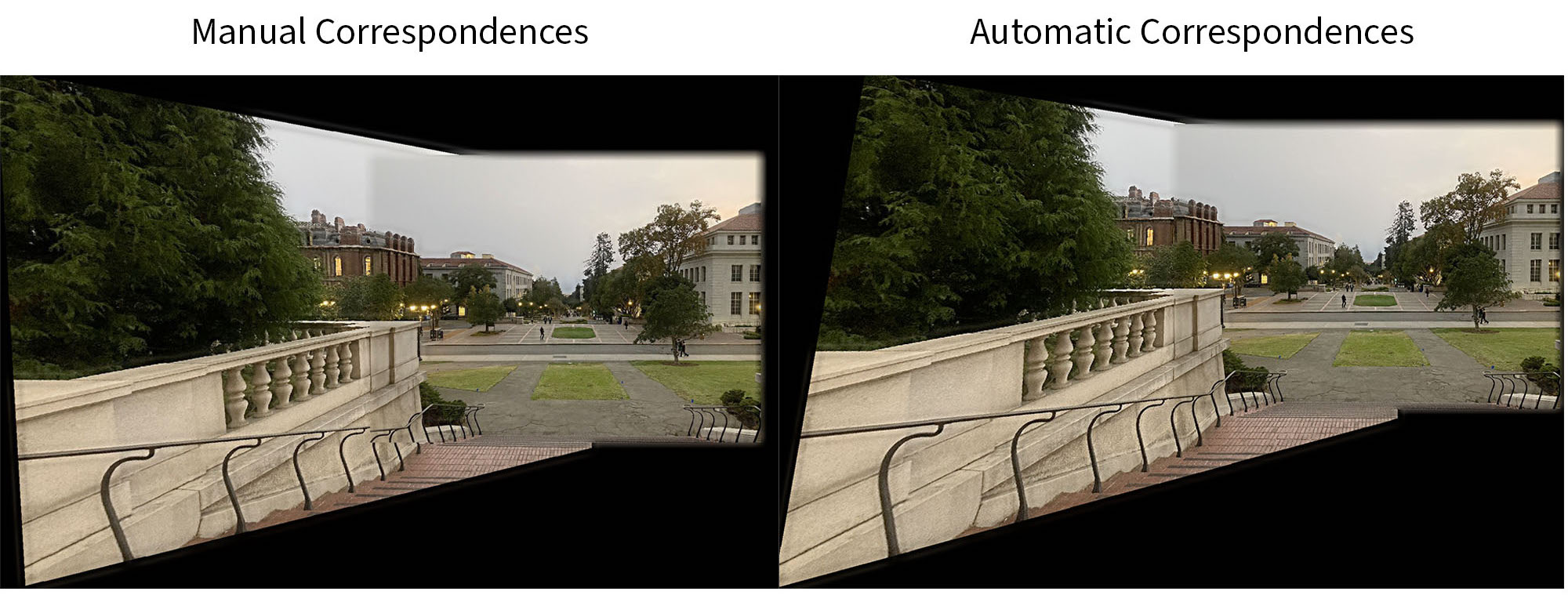
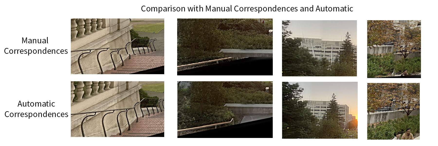
We can see that the results for the sunset panorama look better where the building on the left is (in the manual selection, it was bent). Also in the walkway panorama, the concrete divider on the left looks aligned properly compared to the manual selection version in 4A.

Here are some of the improvements I observed from manually selecting correspondences to having them automatically assigned.

Reflection and what I have learned

I learned about how feature matching works and being able to automate alignment completely which I find interesting since I use colmap regularly. I also learned about RANSAC which could be generalized to other applications as well.